Introduction
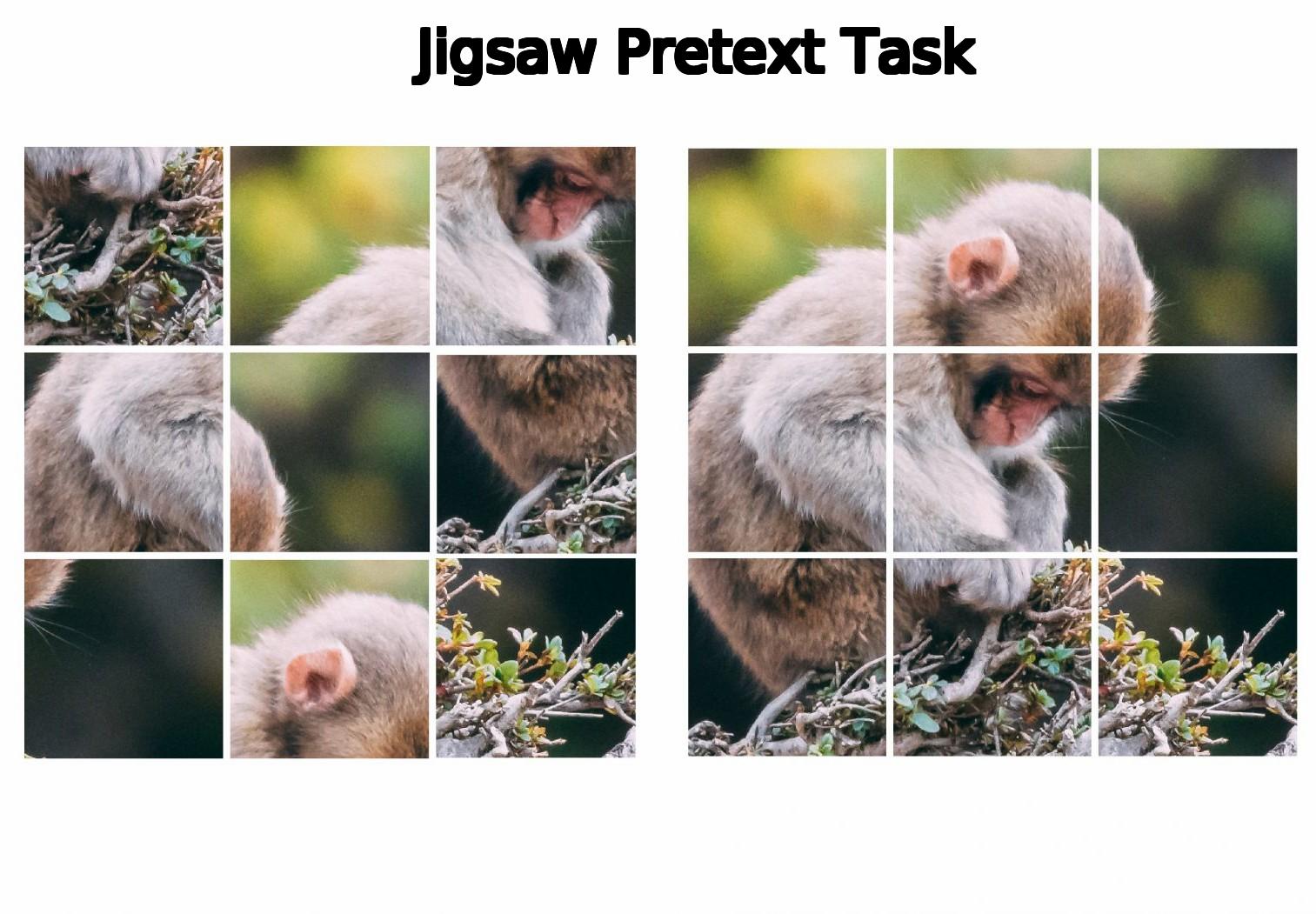
Unsupervised pretraining technqiues can be used to leverage unannotated data to improve a neural network’s ability to solve a task. One way to achieve this is self-supervised learning (SSL), wherein a network is trained to solve a upstream task, whose annotations can be generated automatically. The hidden layers of this network is then used as a feature extractor to solve an unrelated downstream task. This is similar to tranfer learning, wherein a neural network trained to solve a supervised task - say ImageNet - is then finetuned to solve an unrelated downstream task - say COCO. An example of an upstream task is Jigsaw, wherein an image is divided into a grid of sub-images, and the sub-images are shuffled. The network then has to predict the original order of the shuffling.
During the Fall of 2019, I was enrolled in NYU’s Computer Vision course, taught by Prof. Rob Fergus. The topic of the course project was self-supervised learning. We were given almost complete freedom in choosing our project topic. The primary suggestions were:
- Develop techniques - such as a new pretext task - to improve SSL for common downstream tasks like image classification, object detection etc. We were provided a benchmark on the STL-10 dataset, using the VGG-16 neural network.
- Apply current SSL techniques to a new dataset and downstream task.
All projects were conducted in a team of 2 students. We investigated whether pretraining a network on a pretext task in the presence of adversarial noise would improve its performance on a downstream task.
Method and Logic
Presently, supervised pretraining outperforms unsupervised pretraining. For example, consider the ImageNet dataset; A network pretained on ImageNet images and ImageNet annotations significantly outperforms a network pretrained on the ImageNet images to solve the Rotation Prediction pretext task. It is argued that this is due to the current pretext tasks being relatively easy to solve, so the network can solve it without developing useful representations of the input. The state-of-the-art pretext task (on some common downstream tasks) at the time was Image Rotation: An image is rotated by some angle and the network is trained to guess the rotation angle.
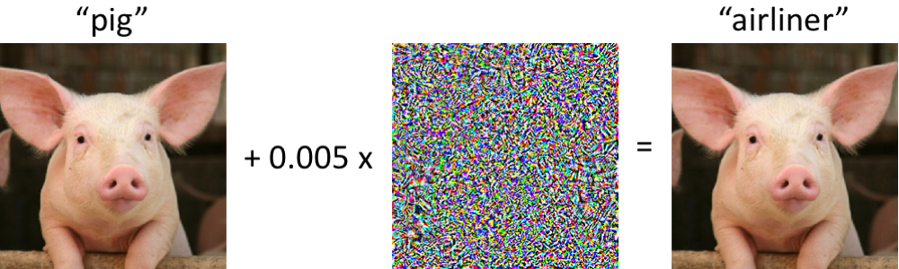
This reminded me of a NeurIPS 2018 tutorial on adversarial robustness in Deep Learning in which the speaker, Aleksander Madry demonstrated how rotating a turtle could cause a state-of-the-art image classifier to mistake it for a rifle. This implies that the rotation transformation makes the classification task more difficult. He goes on to demonstrate how the transformation of an adversarial perturbation of imperceptibly small magnitude can trick the classifier into misclassifying an image. The video can be found here, at time stamp = 12 minutes.
I reasoned that since:
- It is believed that a more difficult pretext task could force a neural network to learn better image representations
- The rotation transformation makes classification more difficult for a neural network
- Pretraining a network on the Rotation Prediction pretext task produces the best image representations
- Adversarial perturbation transformation makes classification significantly more difficult for a neural network, while maintaining the underlying image semantics
then perhaps pretraining a network with the adversarial perturbation transformation would force the neural network to learn significantly better image representations.
Background
Rotation Prediction Pretext task
A rotation angle is chosen from a finite set of angles and the model must guess which angle it is. The Pytorch code will look something like:
class RotationDataSet:
    def __init__(self, get_img_fun, num_images):
        self.get_numpy_img_func = get_img_func
        self.num_images = num_images
        self.choices = [(0, 0), (1, 90), (2, 180), (3, 270)]

    def __len__(self):
        return self.num_images

    def __get_item__(self, idx):
        img = self.get_numpy_img_func(idx)
        annotation, angle = random.sample(self.choices)
        rot_img = numpy.rotate(img, angle)
        return rot_img, annotation
Pretraining a neural network on this task before fine-tuning it on a downstream task can lead to an improvement in performance. It is worth noting that if the downstream task requires features that are rotation invariant, then this could reduce performance. For example, consider the task of classifying a ball as a basket ball or a soccer ball. If an image of a basketball is rotated, then it should till be classified as basketball. Pretraining a neural network on the Rotation Prediction pretext task could reduce performance on ball classification downstream task by producing features that are covariate to the rotation transform.
Adversarial Noise
Adversarial noise with respect to a model and input is a noise generated in a manner that maximises the probability that the model will misclassify the input. Some constraint is usually applied to the noise, so that it cannot modify the true target. For example, suppose we want to generate adversarial noise to trick a network into classifying a picture of a dog as that of a cat. If the noise was unconstrained, it could modify the picture to look like a cat. Then the network would actually be correct in its classification. Perhaps the magnitude of the noise could be restricted to atmost 0.005. More details can be found in the tutorial mentioned above.
Producing features that are invariant to minor perturbations could lead to a more robust classifier that generalises better.
Experiments
We pretrained two VGG-16 networks on the upstream task of guessing the rotation using the unannotated images of the STL-10 dataset. The only difference between them was the noise in the input:
- No noise.
- Adversarial noise of $l-\infty$ norm = 0.01
We compare the performance of the feature extractor of the 2 networks on the STL-10 classification task. For each network, we evaluate a feature extractor trained on top of each of the 5 pooling layers as a feature extractor. A network consisting of a single average pooling layer and linear layer is trained on top of these feature extractors.
The classifiers contain the following number of weights:
| Classifier | Weights |
|---|---|
| POOL-1 | 6400$\times$10 |
| POOL-2 | 3200$\times$10 |
| POOL-3 | 1024$\times$10 |
| POOL-4 | 2048$\times$10 |
| POOL-5 | 512$\times$10 |
Results
We obtianed the following top-1 accuracy on the STL-10 test set:
| Pretraining | POOL-1 | POOL-2 | POOL-3 | POOL-4 | POOL-5 |
|---|---|---|---|---|---|
| Rotation | 48.7% | 60.9% | 60.3% | 59.9% | 47.9% |
| Rotation + adv. noise | 48.5% | 60.1% | 64.6% | 66.5% | 54.9% |
The best model obtained by using our feature extractor achieves an accuracy of 66.5%, while the best model obtained by using the baseline feature extractor achieves an accuracy of 60.9%. Our technique obtains an improvement of 5.6%.
Accuracy Curves
We plotted the train and test accuracy of both the feature extractors as a function of the training epoch.
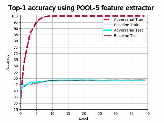
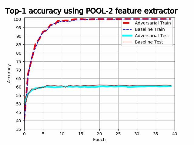
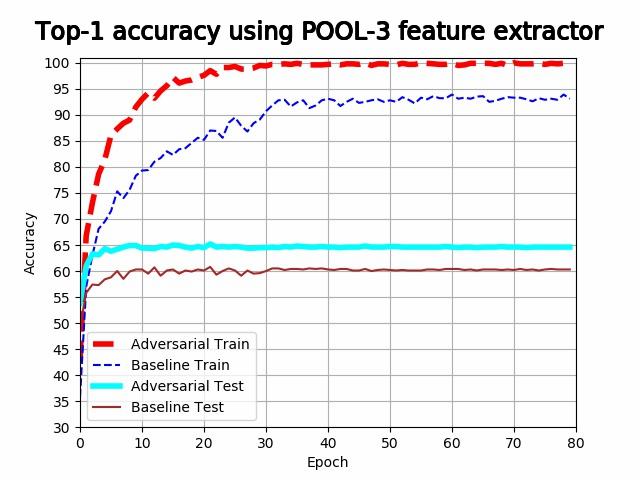
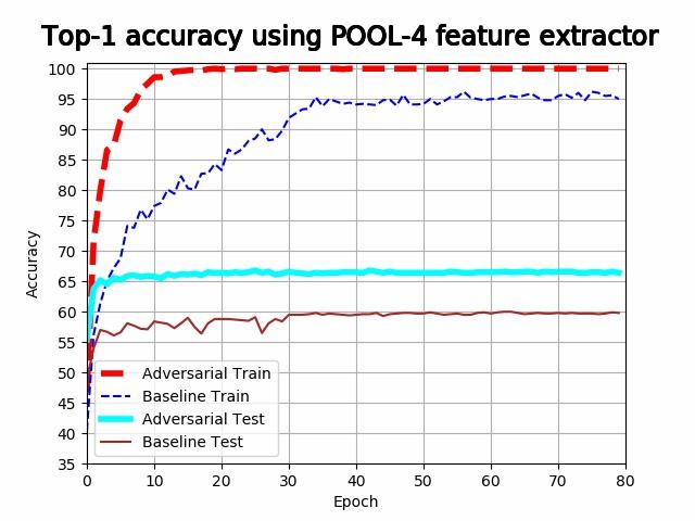
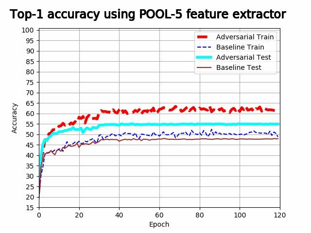
It is evident from the above plots that the models are overfitting when using the first 4 pooling layers, and underfitting when using the last pooling layer. It is evident that both training accuracy and validation accuracy drops at a lower rate in the last 3 plots for the adversarial feature extractors. The feature extractor trained with adversarial noise consistently either outperforms the baseline feature extractor, or performs competitively with it. The best adversarial feature extractor outperforms the best baseline feature extractor with a difference in accuracy of 5.6%.
In the last plot, heavy underfitting is taking place and the test accuracy of the adversarial feature extractor is better than the training accuracy of the baseline feature extractor. In the first 2 plots, heavy overfitting is taking place and the feature extractors perform competitively with each other. This suggests that adversarial noise develops a feature extractor that is more resistant to underfitting.
Conclusion
Our experiments suggest that pretraining a network with adversarial noise develops a feature extractor that is more resistant to underfitting. Perhaps this technique could be used to create a more smaller feature extractor with competitive performance. For example, maybe we could obtain a ResNet-50 feature extractor, with half the number of channels at each hidden layer.
However, the improvement in performance was not as significant as were hoping for, and not nearly enough to justify the huge increase in computational cost. Perhaps we should focus more on developing better pretext tasks, rather than techniques to boost pre-existing pretext tasks.
Updates
20th July 2020: It has been found that adversarial noise improves the feature extractor obtained from pretraining a model on ImageNet. Coincidentally, the findings were published by the professor I mentioned in the logic section. The work can be found here.
Appendix
This section contains additional details regarding the project.
Hyper-parameters
For the 2 experiments stated above, we used the same hyper-parameters as those the benchmarks provided to us:
Pretraining hyper-parameters:
- Weight decay: 0.0001.
- Optimiser: Stochastic Gradient Descent with 0.9 momentum.
- Learning rate: 0.1, divided 10 every 25 epochs.
- Batch size: 128
- Epochs: 60
Adversarial noise is generated through projected gradient descent, with a learning rate of 0.001 and 5 steps per sample. Note that pixel values are in range [0, 1].
Downstream hyper-parameters:
- Weight decay: 0.0005.
- Optimiser: Stochastic Gradient Descent with 0.9 momentum.
- Learning rate: 0.1, divided 10 every 30 epochs.
- Batch size: 64
- Epochs: 120