• Introduction
  • Datset
• Method
  • Logic
  • Model
    • Image Encoder
    • Depth Map Estimator
    • Top View Feature Generator
    • Road Segmenter
    • Object Detector
  • Baseline Model
• Results
• Updates

Introduction

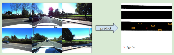
Autonomous vehicles need to estimate its surroundings to plan a safe and efficient route to its destination. The task of Bird Eye View Prediction involves generating a segmentation map of the road and bounding boxes around certain objects - such as cars - as seen from a helicopter above the car.

During the Spring of 2020, I was enrolled in NYU’s Deep Learning course, taught by Prof. Yann Lecun and Prof. Alfredo Canziani. The course project was a competition to develop a model that solves the problem of Bird Eye View Estimation on a novel dataset.

In our project, we focused on leveraging camera geometry and unsupervised depth estimation to construct a “top view representation” of a scene from multiple pictures of the scene. The project was released in the last 4 weeks of the semester, so we had to solve it under significant time constraints.

Datset

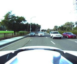
The input is 6 pictures of a scene taken from 6 cameras mounted on top of the car, such that adjacent cameras are at an angle of 60 degrees to each other. The target is a bird eye view, as mentioned above.

A journey consists of 126 scenes of a car’s journey. The dataset is divided into 2 sections:

1. Unannotated Dataset: 106 journeys, with each datapoint containing the 6 images.
2. Annotated DataSet: 28 journeys, with each frame containing the 6 images and its corresponding bird eye view.

A model is not allowed to use preceeding frames during inference. The annotated dataset contains only 2,968 data points. It is infeasible to train a deep neural network using this set alone; The unannotated dataset must also be used, perhaps through self-supervised or semi-supervised learning.

Method

As stated above, we focused on leveraging camera geometry and unsupervised depth estimation to construct a top view representation of the 6 images, from the front view representation of each image.

Logic

Fully convolutional neural networks (FCNN) achieve state-of-the-art performance for typical semantic segmentation and object detection tasks. The main reason for this is the spatial correspondence between the input and output. This leads to the properties of stationarity and locality between input/output pairs, which the 2D convolutional layers of a FCNN exploit. The task of Bird Eye View Prediction does not possess these properties. To describe these properties in brief wrt. image segmentation:

1. Locality: The correlation between input[$i$, $j$] & output[$i+\Delta x$, $j+\Delta y$] decreases as $\vert \Delta x\vert$ or $\vert \Delta y\vert$ increases. For example, the correlation between input[20, 30] & output[21, 31] is more than the correlation between input[20, 30] & output[120, 130]. FCNN exploit this by using convolutional layers with a small kernel size.
2. Stationarity: The correlation between input[$i_1$, $j_1$] & output[$i_2$, $j_2$] is the same as the correlation between input[$i_1+\Delta x$, $j_1+\Delta y$] & output[$i_2+\Delta x$, $j_2+\Delta y$]. For example, the correlation between input[20, 30] & output[40, 50] is similar same as the correlational between input[21, 37] & output[41, 57]. FCNN exploit this through the translational invariance property of convolution operations.

It is easy to notice that unlike image segmentation, bird eye view prediction does not have these properties.

Now let us consider a simpler task to motivate our logic: Rotated Image Segmentation. In this task, the input is an image rotated by some unknown angle. The goal is to generate a segmentation mask of the image before it was rotated.

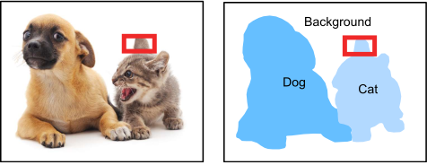
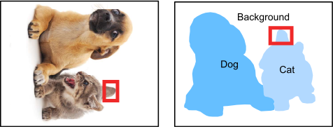
It is easy to see from the above input-output pairs that the task does not possess spatial correspondence between the input and output; Notice the ear of the cat the ear of the cat highlighted in red. Hence, it does have the properties of stationarity and locality.

Instead of training a FCNN to solve this problem, a more reasonable solution might be to train a model using two seperate neural networks. The first network will be trained in a self-supervised manner to predict the rotation of an image. The second network will be trained to solve the image segmentation problem. During inference, we will:

1. Use the first network to predict the rotation of the image.
2. Undo the rotation of the image using any image processing library.
3. Use the second network on the un-rotated image to generate the predicted segmentation map.

Model

The model is divided into 5 sub-models:

1. Image Encoder
2. Depth Map Estimator
3. Top View Feature Generator
4. Road Segmenter
5. Object Detector

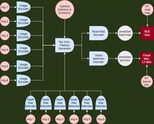
Image Encoder

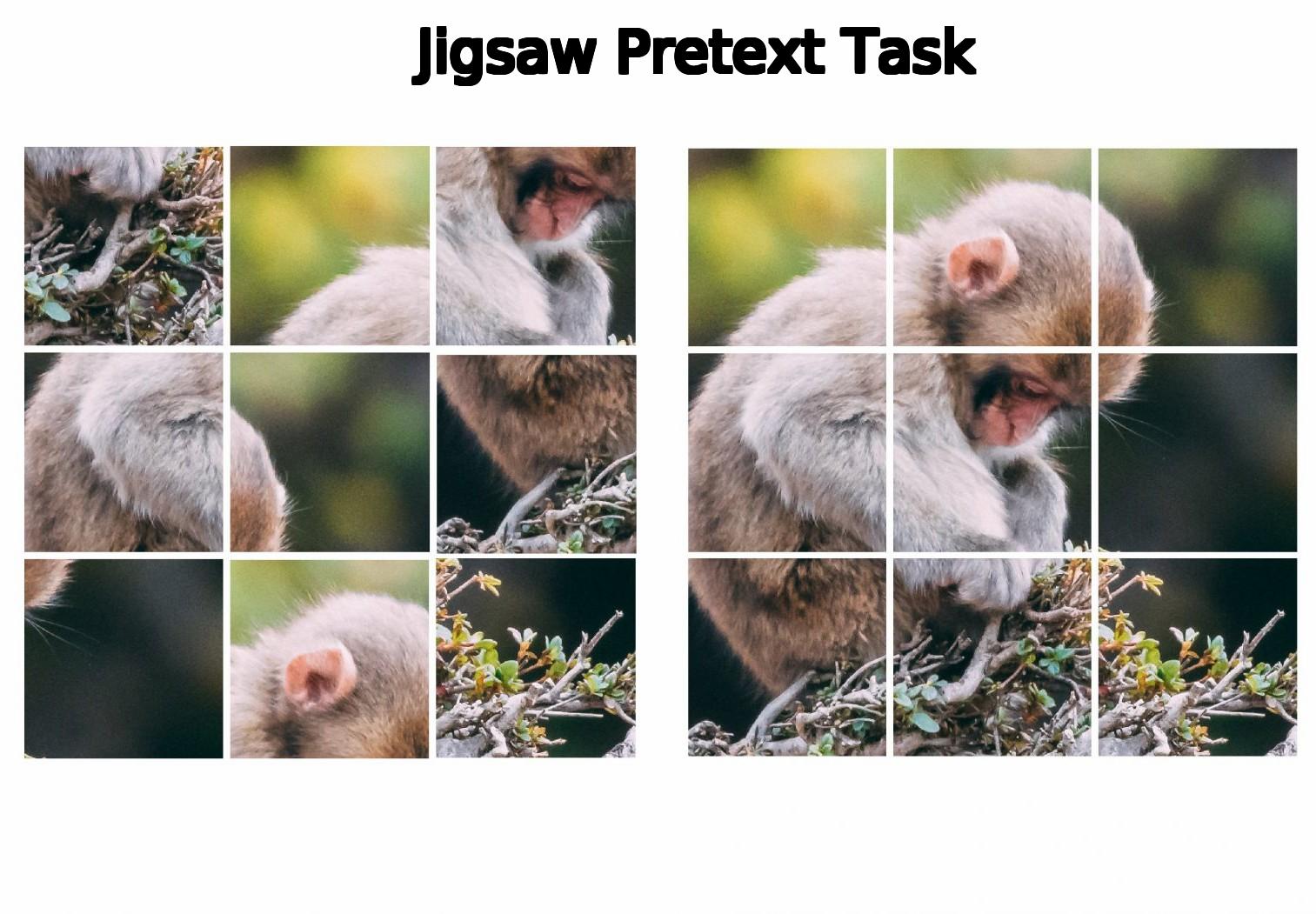
We decided to use self-supervised learning (SSL) to pre-train an image encoder. The image encoder is used to generate a more meaningful representation of the 6 input images. We decided to train the encoder on the jigsaw pretext task. The motivation behind this decision is that the target of the downstream task (Bird Eye View Prediction) is sensitive to the patch-shuffling transformation of jigsaw. Hence, the feature extractor obtained from jigsaw pretraining - whose image representations are covariate to this shuffling transform - might be useful for this task.

We intentionally chose to avoid using the state-of-the-art contrastive SSL techniques - such as MoCo and SimCLR - because the contrastive loss requires a HUGE amount of negative samples. Also, it has been argued that aspects of these techniques are specialised towards the ImageNet dataset, and may not generalise well to others. Due to time and computational constraints, we chose not to risk using such a time consuming technique.

We used the ResNet-18 architecture due to the limited data. However, after reading the landmark ResNet paper, I realised this was a mistake because the depth of the network contributes very little to overfitting: ResNets overfit on ImageNet only when 1,202 layers are used. So we should have explored the possibility of using ResNet-50 and ResNet-34 as the image encoder.

Depth Map Estimator

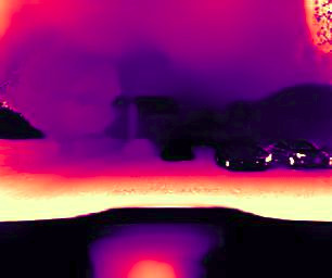
We then trained a ResNet-18 Depth Map Estimator using MonoDepth2 on the unannotated dataset. MonoDepth2 is a unsupervised learning technique used to train a Depth Map Estimator from monocular videos. Since stereo pairs are unavailable, the Depth Map is correct upto some constant factor. There is no guarentee this factor remain constant across images, but the authors found that it usually does.

Since the depth map is accurate upto a constant factor, we conduct a linear transformation on the Depth Map using 2 learnable scalar parameters - $a$, $b$ -, which are optimised during the training of the model. i.e. Depth_scaled = a*Depth_pred + b

Top View Feature Generator

Firstly, it estimates the x-y coordinates of each pixel with respect to the top view using the depth map, camera intrinsics and angle of each camera with respect to the direction the car is facing. One can obtain the 3D coordinates of each pixel from this information using camera geometry. We can then obtain the x-y coordinates of each pixel wrt. the top view:

x, y, z = get_3D_coord(depth_map_list, camera_angle_list, camera_intrinsics_list)
x_out = z
y_out = x

We then produced a top view feature map through a weighted sum of the front view features (image encodings), where the weights are larger for features corresponding to pixels that are closer to the corresponding output location.

($x_s^{\text{top_view}}$, $y_s^{\text{top_view}}$) can easily be obtained using the fact that the output map corresponds to 80m$\times$80m grid around the ego car.

Indexing:

1. $s$: The 6 images
2. $i$, $j$: The spatial dimensions of the FrontViewFeatures.
3. $k$, $l$: The spatial dimensions of the TopViewFeatures.

This was inspired by graphical neural networks. One could consider the closeness of predicted top view coordinates and the estimated top view coordinates to be the degree of connection between Front View Features and Top View features. We implemented efficiently using Pytorch’s Batch Matrix Multiplication subroutine.

Road Segmenter

This was a simple 5-layer FCNN, whose output map is the predicted road segmentation map. It is trained on the target road segmentation map using the binary cross entropy loss function. Inference is conducted by rounding the predicted segmentation map to 0 or 1.

Object Detector

This was a simple 5-layer FCNN, whose output map is the confidence score, class probability, offsets of the anchors. We used focal loss to train the confidence score and class probability, and the smooth L1 loss to train the offsets. During inference, we would conduct non-maximal suppression on the anchor probabilities. It is similar to YOLO.

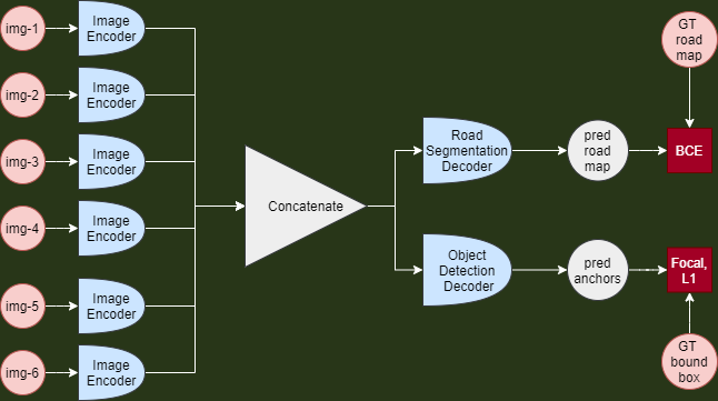
Baseline Model

We also trained a simple baseline model, that is similar of the above model, except it combines the 6 image encodings by simply concatenating them along the channel dimension, instead of using a Depth Map Estimator and Top View Feature Generator.

Results

Unfortunately, the results we obtained from the network were terrible. Our benchmark model significantly outperformed it. We learned (too late) that unsupervised monocular depth estimation operates under the assumption that the scene is mostly static with the camera moving. Hence, cars moving with the same velocity as the ego car are predicted to be at infinite depth.

We ended up submitting the benchmark model, which achieved average results. In hindsight, we should have stuck to an approach we had prior experience in, especially considering the time and computational restrictions.

Updates

10th June 2020: I began working in the instructors’ research group on this task. In particular, we are trying to achieve competitive performance on the Waymo Open Dataset using a fraction of its annotations.

• Deep-Learning (5)

• Autonomous-Vehicles (3) ,
• Computer-Vision (3) ,
• Deep-Learning (5) ,
• Machine-Learning (5) ,
• Pytorch (5) ,
• Python (5) ,
• Unsupervised-Learning (2) ,
• Self-supervised-Learning (2)