Introduction
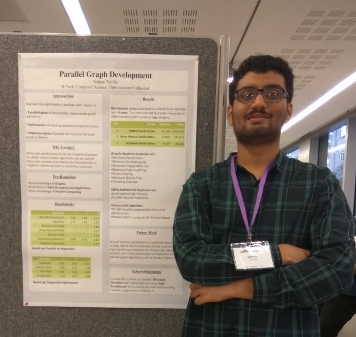
The project of Prediction and Policy learning Under Uncertainty tackles the problem of training an autonomous agent to drive through dense traffic. The driving agent has access to the segmented top view (bird’s eye view) of its surroundings. The project was published in ICLR 2019, by Mikael Henaff (Facebook AI Research), Prof. Alfredo Canziani (NYU) and Prof. Yann Lecun (Facebook AI Research, NYU). Upon completing NYU’s Deep Learning course - mentioned in a previous post - I was allowed to join the instructor’s research group.
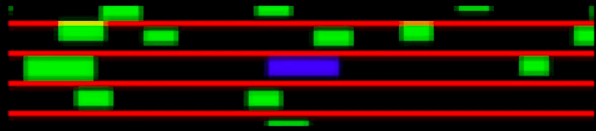
The above figure represents the segmented top view available to an agent. The blue, green, red pixels represent the agent car, back-ground cars, lane markings respectively.
Since NYU’s budget and lawyers won’t allow us to train an autonomous agent by trial and error on the highway (Model-free Reinforcement Learning), pre-recorded traffic is used to train a World Model (simulator) that approximates a highway stretch and the agent is trained in the World Model (Offline Model-based Reinforcement Learning). The performance of an agent is evaluated by its ability to navigate through a pre-recorded 200m highway stretch. For a more detailed explaination, please refer the official video summary.
I made two contributions to this project:
- I implemented a program to test an agent on a longer highway stretch, using multiple smaller highway stretches.
- I improved the performance of the driving agent by improving the World Model.
This post will focus on the latter, but touch on the former at the end.
Method
I investigated the possibility of improving the World Model by injecting more inductive bias into it, a task a PhD student had worked on. While examining the World Model, I noticed the model’s final activation function was sigmoid. The pixels of the segmented top view are binary ($0$ or $1$), but the output of the sigmoid is biased against binary values. This could lead to a discrprency between the distribution of the true top view images, and the simulated top view images. I created a histogram of the pixel values of the true top view images and the simulated top view images:
| Range | True Images | Simulated Images |
|---|---|---|
| 0.00 to 10^-9 | 77.05% | 0.00% |
| 10^-9 to 0.10 | 2.53% | 79.26% |
| 0.10 to 0.20 | 6.74% | 6.19% |
| 0.20 to 0.30 | 1.23% | 0.89% |
| 0.30 to 0.40 | 0.07% | 1.14% |
| 0.40 to 0.50 | 0.28% | 1.10% |
| 0.50 to 0.60 | 0.89% | 0.69% |
| 0.70 to 0.80 | 1.30% | 0.83% |
| 0.80 to 0.90 | 6.41% | 6.48% |
| 0.90 to 1-10^-9 | 0.96% | 3.38% |
| 1-10^-9 to 1.00 | 2.48% | 0.00% |
As you can see, most of the pixels of the true images are zero, but most of those in the simulated images are in the range ($0.9, 0.1$). Due to the highly non-linear nature of deep neural networks, this minor discreprency might affect the performance of the driving agent.
Surprisingly, there are a few non-binary values in the true image, around the cars and lanes. This was a result of downsampling the image. Since sigmoid has high gradient in the region between 0 and 1, closer to 0.5 (and the Policy Model is trained using back-propagation), the policy model might be relying on those pixels for gradient signal instead of the pixels whose values are 1.
I then compared the actions (acceleration and steering) of the driving agent during the validation phase of policy training, after it was provided a simulated image, versus a simulated image whose pixels having the value ($0, 0.1$), ($0.9, 1$) were set to $0$, $1$ respectively. Recall that the policy is trained using the simulated images created by the World Model.
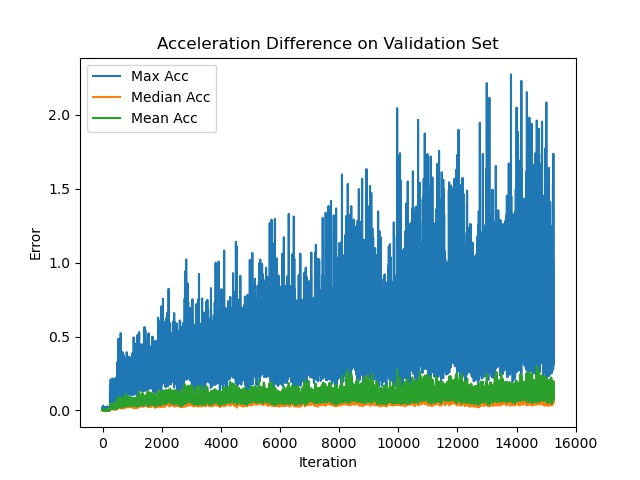
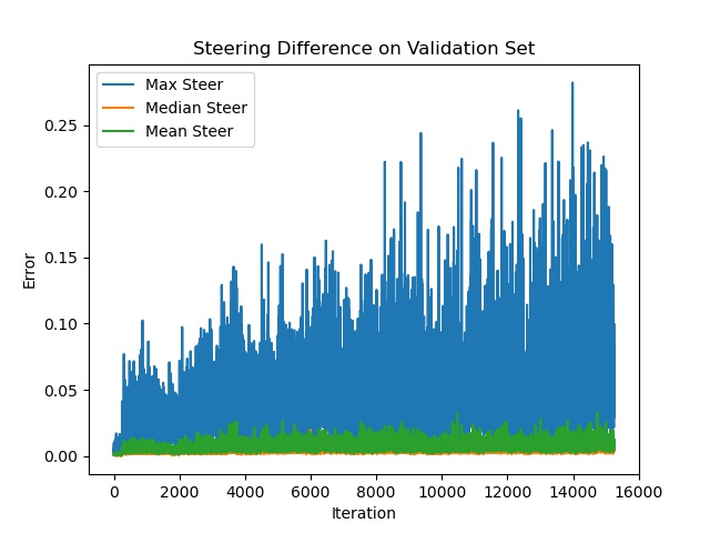
The difference in acceleration could be as large as 2m/s, which could easily cause a crash in dense traffic.
Experiment
I created a Thresholded World Model by making a simple modification to the original World Model: Set its output pixels in the range ($0, 0.1$) to $0$, and those in the range ($0.9, 1$) to $1$, while preserving a gradient. Some might consider this to be a hacky and naive way to go about it, but it gets results quickly. One of the lessons I had learned from the Deep Learning Course Project is to validate your idea quickly before investing significant time in it - My initial plan was to create a novel activation function and a novel autograd scheme, in which each node of the computational graph has a left-gradient and right-gradient …….
The code looks something like this:
import torch
import torch.nn as nn

# Pyotch Autograd function
class Threshold(torch.autograd.Function):
    @staticmethod
    def forward(ctx, input, cut_off):
        output = input.clone()
        output[output <= cut_off] = 0
        output[output >= 1-cut_off] = 1
        return output, None

    @staticmethod
    def backward(ctx, grad_output):
        return grad_output.clone()


class ThresholdedWorldModel(nn.Module):
    def __init__(self, world_model, cut_off):
        super(ThresholdedWorldModel, self).__init__()
        self.world_model = world_model
        self.cut_off = cut_off
        self.policy_training = False

    def forward(self, current_state, action):
        next_state = self.world_model(current_state, action)
        if self.policy_training:
            next_state = Threshold.apply(next_state, self.cut_off)
        return next_state

    def train_policy(self):
        self.policy_training = True
    def train_self(self):
        self.policy_training = False
This could be viewed as modifying the sigmoid activation function to thresholded sigmoid, which could be described as:
I also investigated the effect of discretizing the output of the World Model by projecting each pixel value to the set of pixel values found in the test images.
The code looks something like this:
import torch
import torch.nn as nn

# Pyotch Autograd function
class Discretize(torch.autograd.Function):
    @staticmethod
    def forward(ctx, input, codes):
        input = input.unsqueeze(-1)
        codes = codes.view(1, 1, 1, 1, -1)
        distance = torch.abs(inputs - codes)
        min_ind = torch.argmin(distance, axis = -1)
        output = codes[min_ind]
        return output

    @staticmethod
    def backward(ctx, grad_output):
        return grad_output.clone()


class DiscretizedWorldModel(nn.Module):
    def __init__(self, world_model):
        super(ThresholdedWorldModel, self, pixel_codes).__init__()
        self.world_model = world_model
        self.pixel_codes = pixel_codes
        self.policy_training = False

    def forward(self, current_state, action):
        next_state = self.world_model(current_state, action)
        if self.policy_training:
            next_state = Discretize.apply(next_state, self.pixel_codes)
        return next_state

    def train_policy(self):
        self.policy_training = True
    def train_self(self):
        self.policy_training = False
I conducted the following experiments:
- Evaluate agent trained in a Thresholded World Model.
- Evaluate the above two agents, but downsample the test images
- Adjust the threshold cut-off, based on the findings of the above two experiments, and evaluate it.
- Evaluate agent trained in a Discretized World Model.
Results
Note that the performance of an agent varies with hyper-parameters, random seed and training steps; Please refer to the evaluation notebook for more information. The hyper-parameters are tuned for training the agents using a regular World Model.
1. Thresholded World Model
I evaluated an agent that was trained in a Thresholded World Model and compared it to one trained in a Regular World Model.
| Training Steps | Regular World Model | Thresholded World Model |
|---|---|---|
| 5,000 | 40.5% | 43.0% |
| 10,000 | 54.2% | 73.6% |
| 15,000 | 65.2% | 50.6% |
| 20,000 | 27.6% | 72.0% |
| 25,000 | 68.1% | 71.5% |
| 30,000 | 71.5% | 67.4% |
| 35,000 | 61.9% | 72.0% |
| 40,000 | 73.1% | 64.2% |
| 45,000 | 71.5% | 77.2% |
| 50,000 | 74.0% | 75.2% |
| 55,000 | 70.4% | 73.4% |
| 60,000 | 72.7% | 74.0% |
| 65,000 | 75.4% | 75.9% |
| 70,000 | 72.9% | 74.3% |
| 75,000 | 66.0% | 62.2% |
| Mean | 64.3% | 68.4% |
| Std | 13.2% | 9.4% |
| Best | 75.4% | 77.2% |
As you can see from the above table, the agent trained using a Thresholded World Model outperforms the one trained using a regular World Model in terms of average success rate, best success rate and variance. This seems like a significant improvement, but it is worth noting that the performance of an agent varies with hyper-parameters, random seed and training steps. It is worth noting though that the agent trained in a Thresholded World Model outperforms the other 11 - 4 times, when evaluated at the same time step.
2. Billinear Downsampling vs Nearest Downsampling
I again evaluated the above two agents, but downsampled the test images using Nearest Downsampling instead of Billinear Downsampling.
| Training Steps | Regular World Model | Thresholded World Model |
|---|---|---|
| 5,000 | 29.9% | 42.4% |
| 10,000 | 35.8% | 62.0% |
| 15,000 | 59.0% | 39.0% |
| 20,000 | 33.5% | 64.7% |
| 25,000 | 58.1% | 65.4% |
| 30,000 | 68.1% | 64.9% |
| 35,000 | 52.6% | 70.9% |
| 40,000 | 63.5% | 56.0% |
| 45,000 | 70.1% | 70.2% |
| 50,000 | 67.4% | 39.0% |
| 55,000 | 67.9% | 68.3% |
| 60,000 | 60.8% | 72.9% |
| 65,000 | 66.5% | 68.1% |
| 70,000 | 55.9% | 74.9% |
| 75,000 | 60.4% | 56.7% |
| Mean | 56.6% | 61.0% |
| Std | 12.7% | 11.6% |
| Best | 70.1% | 74.9% |
Once again, the model trained using a Thresholded World Model outperforms one trained using a Regular World Model.
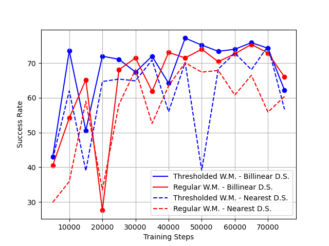
As you can see from Figure 4, applying Nearest downsampling to the Top View images at test time usually leads to a significant decrease in performance, implying that the driving agent relies on the soft pixels at the edge of a car to make its decisions, instead of binary pixels interior to the cars.
3. Adjust Threshold Cut-off
The experiment using Nearest downsampling found that the soft-pixels of the test images help the agent choose a better action. So perhaps too much thresholding decrease the performance of the agent. I found that the smallest non-zero pixel value in the test images is $0.0039$, and trained the agent in a Thresholded World Model with a cut-off of $0.001$ instead of $0.1$.
| Training Steps | Threshold cut-off = 0.1 | Thresholded cut-off = 0.001 |
|---|---|---|
| 5,000 | 43.0% | 49.2% |
| 10,000 | 73.6% | 75.8% |
| 15,000 | 50.6% | 65.6% |
| 20,000 | 72.0% | 66.8% |
| 25,000 | 71.1% | 69.3% |
| 30,000 | 67.4% | 73.1% |
| 35,000 | 72.0% | 79.0% |
| 40,000 | 64.2% | 76.5% |
| 45,000 | 77.2% | 73.8% |
| 50,000 | 75.2% | 65.1% |
| 55,000 | 73.4% | 62.9% |
| 60,000 | 74.0% | 70.6% |
| 65,000 | 75.9% | 75.2% |
| 70,000 | 74.3% | 69.5% |
| 75,000 | 62.2% | 69.2% |
| Mean | 68.40% | 69.44% |
| Std | 9.49% | 7.03% |
| Best | 77.2% | 79.0% |
Using a smaller cut-off to avoid thresholding soft pixel values that are present in the test image seems to further improve performance in terms of average success rate, best success rate and variance. But once again, it is difficult to judge its statistical significance.
Unless stated otherwise, Thresholded World Models will hence-forth use a cut-off of $0.001$.
4. Discretized World Model
| Training Steps | Regular World Model | Thresholded World Model | Discretized World Model |
|---|---|---|---|
| 5,000 | 40.5% | 49.2% | 44.2% |
| 10,000 | 54.2% | 75.8% | 31.0% |
| 15,000 | 65.2% | 65.6% | 59.4% |
| 20,000 | 27.6% | 66.8% | 74.7% |
| 25,000 | 68.1% | 69.3% | 69.2% |
| 30,000 | 71.5% | 73.1% | 74.3% |
| 35,000 | 61.9% | 79.0% | 67.4% |
| 40,000 | 73.1% | 76.5% | 70.9% |
| 45,000 | 71.5% | 73.8% | 73.1% |
| 50,000 | 74.0% | 65.1% | 77.9% |
| 55,000 | 70.4% | 62.9% | 62.6% |
| 60,000 | 72.7% | 70.6% | 73.6% |
| 65,000 | 75.4% | 75.2% | 73.3% |
| 70,000 | 72.9% | 69.5% | 66.5% |
| 75,000 | 66.0% | 69.2% | 64.3% |
| Mean | 64.33% | 69.44% | 65.49% |
| Std | 13.21% | 7.03% | 12.21% |
| Best | 75.4% | 79.0% | 77.9% |
The agent trained in Discretized World Model outperforms the one trained in a Regular World Model terms of average success rate, best success rate and variance, by a slim margin. The agent trained in a Thresholded World Model outperforms the others.
Conclusion
It is possible that the final sigmoid activation function of the World Model likely biases it in a manner that hurts the performance of the driving agent. Firstly, it causes a discreprency in pixel values since true images have binary pixel values and sigmoid is biased against binary values. Secondly, since sigmoid has lesser gradient at its extreme points, the agent trained in the World Model may rely on the soft pixels at the edge of the car to choose its actions.
Thresholding the output of the World Model - which effectively modifies the final activation function - improved the performance of the driving agent, but it is worth noting that the performance of an agent varies with the training steps, hyperparameters and random seed, so it is difficult to judge its statistical significance.
Infinite Testing
In this section, I will briefly touch upon the contributions I made regarding the testing methodology. Previously, the performance on an agent was judged by the frequency with which it navigated through a 200m highway stretch. I developed software to combine multiple highway stretches so the car entered the next stretch after completing the current one. The main challenge was ensuring consistency when the car leaves one stretch and enters the other. The main issue I faced is that the data is noisy at the highway end-points: Cars appear and disappear abruptly.
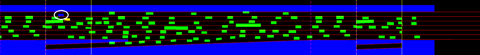
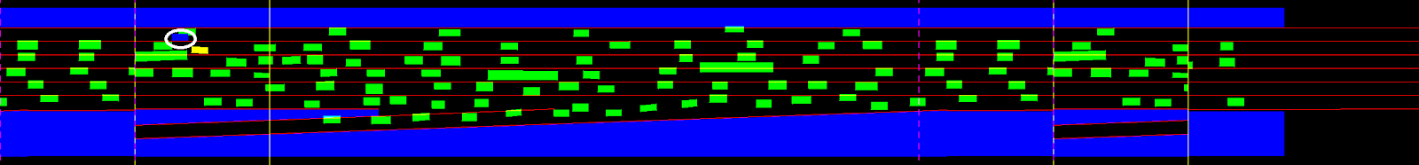
The ego car is near the top left corner of the image with a white circle drawn around it. As you can see from the above figure, a crash occured due to the noise in the pre-recorded trajectories. To remedy, this create a safe zone around the ego car. If a background car abruptly appears inside a safe zone, then the car will be invisible to the ego car and colliding with it will not result in a crash, until it leaves the safe zone.
I evaluated the SotA driving agents in terms of distance traveled and its ability to avoid crashing 5 minutes (3,000 time steps). I initially set the safe zone to the space occupied by the ego car.
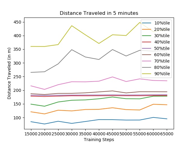
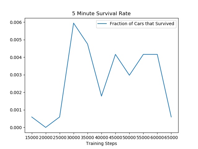
As expected, the performance is very poor, with a peak survival rate of 0.6%. At least 20% of the crashes - 40%tile to 60%tile - occur when the car transitions from the end of one highway stretch to the beginning of the second. Recall that a highway stretch is approximately 200m long.
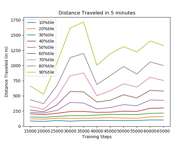
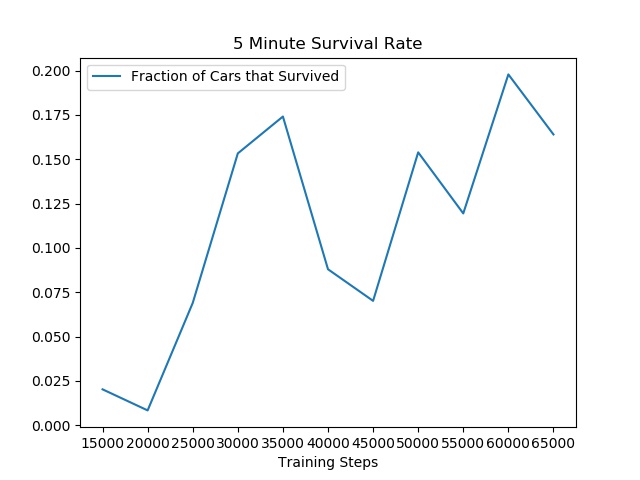
The driving agent achieves a peak survival rate of 20%, even with this generous relaxation.